Exponential Growth and Decay
Exponential Functions
An exponential function with base b is defined by f (x) = abx
where a ≠0, b > 0 , b ≠1, and x is any real number.
The base, b, is constant and the exponent, x, is a variable.
Notice: The variable x is an exponent. As such, the graphs of these functions are not straight lines. In a straight line, the “rate of change” is the same across the graph. In these graphs, the “rate of change” increases or decreases across the graphs.
Observe how the graphs of exponential functions change based upon the values of a and b:
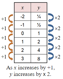
In the following example, a = 1 and b = 2.
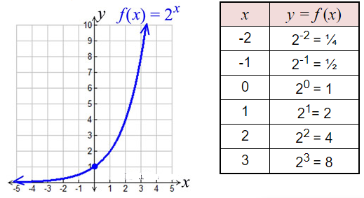
Features (for this graph):
- the domain is all Real numbers.
- the range is all positive real numbers (not zero).
- graph has a y-intercept at (0,1). Remember any number to the zero power is 1.
- when b > 1, the graph increases. The greater the base, b, the faster the graph rises from left to right.
- when 0 < b < 1, the graph decreases.
- has an asymptote (a line that the graph gets very, very close to, but never crosses or touches). For this graph the asymptote is the x-axis (y = 0).
Growth and Decay
Many real world phenomena can be modeled by functions that describe how things grow or decay as time passes. Examples of such phenomena include the studies of populations, bacteria, the AIDS virus, radioactive substances, electricity, temperatures and credit payments, to mention a few.
Any quantity that grows or decays by a fixed percent at regular intervals is said to possess exponential growth or exponential decay.
At the Algebra level, there are two functions that can be easily used to illustrate the concepts of growth or decay in applied situations. When a quantity grows by a fixed percent at regular intervals, the pattern can be represented by the functions,
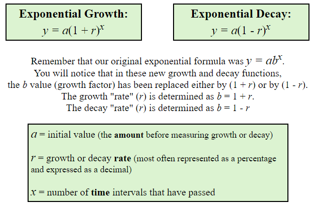
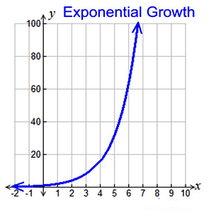
In exponential growth, the quantity increases, slowly at first, and then very rapidly. The rate of change increases over time. The rate of growth becomes faster as time passes. This rapid growth is what is meant by the expression “increases exponentially”.
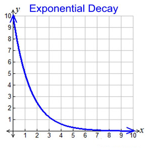
In exponential decay, the quantity decreases very rapidly at first, and then more slowly. The rate of change decreases over time. The rate of decay becomes slower as time passes.
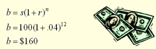
Example: A bank account balance, b, for an account starting with s dollars, earning an annual interest rate, r, and left untouched for n years can be calculated as b = s(1 + r)n (an exponential growth formula). Find a bank account balance to the nearest dollar, if the account starts with $100, has an annual rate of 4%, and the money left in the account for 12 years.
We will now examine rate of growth and decay in a three step process. We will (1) build a chart to examine the data and “see” the growth or decay, (2) write an equation for the function, and (3) prepare a scatter plot of the data along with the graph of the function.
Consider these examples of growth and decay:
Growth:
Cell Phone Users In 1985, there were 285 cell phone subscribers in the small town of Centerville. The number of subscribers increased by 75% per year after 1985. How many cell phone subscribers were in Centerville in 1994? (Don’t consider a fractional part of a person.)
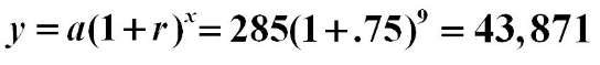
Therefore, there were 43,871 subscribers in 1994.
Growth by doubling:
One of the most common examples of exponential growth deals with bacteria. Bacteria can multiply at an alarming rate when each bacteria splits into two new cells, thus doubling. For example, if we start with only one bacteria which can double every hour, by the end of one day we will have over 16 million bacteria.
Let’s examine the graph of our scatter plot and function. To the left of the origin we see that the function graph tends to flatten, but stays slightly above the x-axis. To the right of the origin the function graph grows so quickly that it is soon off the graph. The rate at which the graph changes increases as time increases.
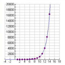 When we can see larger y-values, we see that the growth still continues at a rapid rate. This is what is meant by the expression “increases exponentially”.
Note: In reality, exponential growth does not continue indefinitely. There would, eventually, come a time when there would no longer be any room for the bacteria, or nutrients to sustain them. Exponential growth actually refers to only the early stages of the process and to the manner and speed of the growth.
Decay:
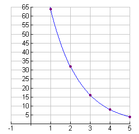
Tennis Tournament Each year the local country club sponsors a tennis tournament. Play starts with 128 participants. During each round, half of the players are eliminated. How many players remain after 5 rounds?
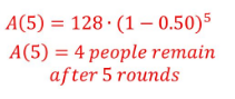
Notice the shape of this graph compared to the graphs of the growth functions.
Decay by half-life:
The pesticide DDT was widely used in the United States until its ban in 1972. DDT is toxic to a wide range of animals and aquatic life, and is suspected to cause cancer in humans. The half-life of DDT can be 15 or more years. Half-life is the amount of time it takes for half of the amount of a substance to decay. Scientists and environmentalists worry about such substances because these hazardous materials continue to be dangerous for many years after their disposal.
For this example, we will set the half-life of the pesticide DDT to be 15 years.
Let’s mathematically examine the half-life of 100 grams of DDT.
Let’s examine the scatter plot and the function. At 0 the y-intercept is 100. To the right of the origin we see that the graph declines rapidly and then tends to flatten, staying slightly above the x-axis. The rate of change decreases as time increases.
When we zoom in on the flattened area of the graph, we see that the graph does stay above the x-axis. This makes sense because we could not have a “negative” number of grams of DDT leftover.
Exponential growth and decay are mathematical changes. The rate of the change continues to either increase or decrease as time passes. In exponential growth, the rate of change increases over time – the rate of the growth becomes faster as time passes. In exponential decay, the rate of change decreases over time – the rate of the decay becomes slower as time passes. Since the rate of change is not constant (the same) across the entire graph, these functions are not straight lines.