Equations and Graphing
There are several ways to graph a straight line given its equation.
The basic method of graphing a straight line is to prepare a table (or T-chart) of x-values and y-values to obtain points, and to plot these points. When dealing with straight lines, with constant (never changing) slopes, only a few points (actually only two) are needed to produce the line.
Graphing with a table or chart (T-chart):
Choosing Chart Values: When choosing x-values for the chart, choose both positive and negative values. This is a good habit to develop for dealing with other types of graphs. Also choose at least three points. Yes, two points will determine a line, but if you make a mistake you will never know since you created a straight line (but the wrong one). If you make a mistake with one of three points, you are more likely to see that the points do not form a straight line.
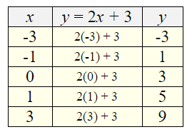
Example: Graph y = 2x + 3
We are going to choose 5 x-values for our chart.
You may need to rearrange your equation until is starts with “y = “.
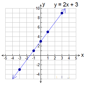
Plot (x,y) on the coordinate grid to reveal the graph. Be sure to include all of the “nice” graph items, such as labeling the x and y axes, labeling the scales on the axes (at least to 1 unit on both axes), and placing the statement of the equation on the graph.
Graphing using the Slope – Intercept Form:
Linear equations often appear in the form y = mx + b. In this form, m is the slope of the line and b is the y-intercept (where the line crosses the y-axis.), thus its name “Slope – Intercept Form”.
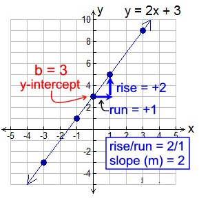
Example 1: Graph y = 2x + 3.
We can see that y = 2x + 3 is in the Slope – Intercept Form, with m = 2 and b = 3.
y = mx + b
y = 2x + 3
We could have graphed this line without completing a table or chart, by simply using where the line crosses the y-axis and its slope.
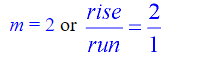
Start by plotting the y-intercept (b): b = 3 or (0,3).
Then, from that point, apply the slope (m):
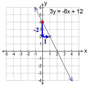
Example 2: Graph 3y = -6x + 12
At first glance, it appears that this line is not a candidate for the Slope – Intercept Form. But, if we use our algebra skills, we can re-write this equation so that it fits the Slope – Intercept Form of y = mx + b.
We need the equation to be “y = “, not “3y =”.
If we divide ALL terms by 3, we will get the equation we need.
y = -2x + 4
We now have the form y = mx + b.
The y-intercept (b) is +4. Plot this point first, (0,4).
The slope (m) is -2. So the rise/run = -2/1.
Starting at the y-intercept, go down 2 units and right 1 unit. This new location (1,2) is another point on the line. Draw the line.
Graphing Tidbits
If a point lies on a line, its coordinates make the equation true.
(2, 1) in on the line y = 2x – 3 because 1 = 2(2) – 3
Before graphing a line, be sure that your equation starts with “y=”.
To graph 6x + 2y = 8
rewrite the equation: 2y = -6x +8
y = -3x + 4
Now graph the line using either slope intercept method or chart method.
The x-coordinate may be called the abscissa.
The y-coordinate may be called the ordinate.
An Intercept Graphing Method:
This graphing approach is particularly useful when your equation is in standard form, Ax + By = C.
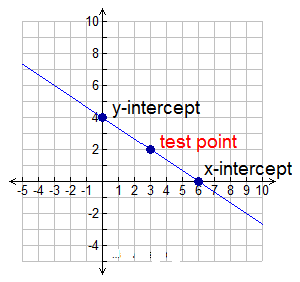
Graph 2x + 3y = 12
Yes, you can re-write this equation and use a table or the slope-intercept method for graphing. But, there is another option which may be easier to use in this situation.
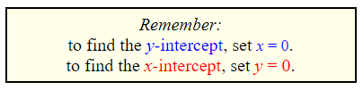
We are going to obtain the x-intercept and the y-intercept. We will then choose one additional test point (to avoid possible errors) and show that all three points form a line.
If you want to organize your work, you can set up a small table or chart.
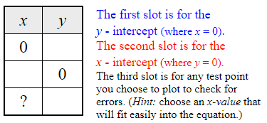
Here is the completed chart for the graph seen above.
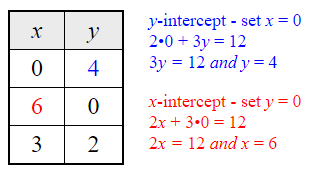
We chose x = 3 to create the test point.
2•3 + 3y = 12
6 + 3y = 12
3y = 6
y = 2