What is Cumulative Frequency Curve or the Ogive in Statistics
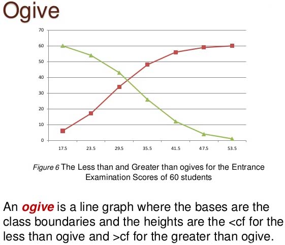
First we prepare the cumulative frequency table, then the cumulative frequencies are plotted against the upper or lower limits of the corresponding class intervals. By joining the points the curve so obtained is called a cumulative frequency curve or ogive.
There are two types of ogives :
- Less than ogive : Plot the points with the upper limits of the class as abscissae and the corresponding less than cumulative frequencies as ordinates. The points are joined by free hand smooth curve to give less than cumulative frequency curve or the less than Ogive. It is a rising curve.
- Greater than ogive : Plot the points with the lower limits of the classes as abscissa and the corresponding Greater than cumulative frequencies as ordinates. Join the points by a free hand smooth curve to get the “More than Ogive”. It is a falling curve.
When the points obtained are joined by straight lines, the picture obtained is called cumulative frequency polygon.
Less than ogive method:
To construct a cumulative frequency polygon and an ogive by less than method, we use the following algorithm.
Algorithm
Step 1 : Start with the upper limits of class intervals and add class frequencies to obtain the cumulative frequency distribution.
Step 2 : Mark upper class limits along X-axis on a suitable scale.
Step 3 : Mark cumulative frequencies along Y-axis on a suitable scale.
Step 4 : Plot the points (xi, fi) where xi is the upper limit of a class and fi is corresponding cumulative frequency.
Step 5 : Join the points obtained in step 4 by a free hand smooth curve to get the ogive and to get the cumulative frequency polygon join the points obtained in step 4 by line segments.
More than ogive method:
To construct a cumulative frequency polygon and an ogive by more than method, we use the following algorithm.
Algorithm
Step 1 : Start with the lower limits of the class intervals and from the total frequencysubtract the frequency of each class to obtain the cumulative frequency distribution.
Step 2 : Mark the lower class limits along X-axis on a sutiable scale.
Step 3 : Mark the cumulative frequencies along Y-axis on a suitable scale.
Step 4 : Plot the points (xi, fi) where xi is the lower limit of a class and fi is corresponding cumulative frequency.
Step 5 : Join the points obtained in step 4 by a free hand smooth curve to get the ogive and to get the cumulative frequency polygon join these points by line segments
Read More:
- Classmark and Discrete Frequency Distribution
- Cumulative Frequency in statistics
- RS Aggarwal Class 10 Solutions Mean, Median, Mode of Grouped Data
- RS Aggarwal Class 9 Solutions Statistics
Cumulative Frequency Curve or the Ogive Example Problems with Solutions
Example 1: Draw a less than ogive for the following frequency distribution :
| I.Q. | Frequency |
| 60 – 70 | 2 |
| 70 – 80 | 5 |
| 80 –90 | 12 |
| 90 – 100 | 31 |
| 100 – 110 | 39 |
| 110 – 120 | 10 |
| 120 – 130 | 4 |
Find the median from the curve.
Solution: Let us prepare following table showing the cumulative frequencies more than the upper limit.
| Class interval (I. Q) | Frequency (f) | Cumulative frequency |
| 60 – 70 | 2 | 2 |
| 70 – 80 | 5 | 2 + 5 = 7 |
| 80 –90 | 12 | 2 + 5 + 12 = 19 |
| 90 – 100 | 31 | 2 + 5 + 12 + 31 = 50 |
| 100 – 110 | 39 | 2 + 5 + 12 + 31 + 39 = 89 |
| 110 – 120 | 10 | 2 + 5 + 12 + 31 + 39 + 10 = 99 |
| 120 – 130 | 4 | 2 + 5 + 12 + 31 + 39 + 10 + 4 = 103 |
Less than ogive :
I.Q. is taken on the x-axis. Number of students are marked on y-axis.
Points (70, 2), (80, 7), (90, 19), (100, 50), (110, 89), (120, 99), (130, 103), are plotted on graph paper and these points are joined by free hand. The curve obtained is less than ogive.
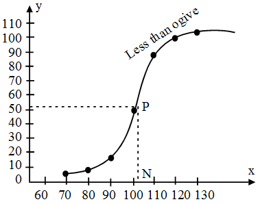
The value \(\frac{N}{2}\) = 51.5 is marked on y-axis and from this point a line parallel to x-axis is drawn. This line meets the curve at a point P. From P draw a perpendicular PN to meet x-axis at N. N represents the median.
Here median is 100.5.
Hence, the median of given frequency distribution is 100.5
Example 2: The following table shows the daily sales of 230 footpath sellers of Chandni Chowk.
| Sales in Rs. | No. of sellers |
| 0 – 500 | 12 |
| 500 – 1000 | 18 |
| 1000 – 1500 | 35 |
| 1500 – 2000 | 42 |
| 2000 – 2500 | 50 |
| 2500 – 3000 | 45 |
| 3000 – 3500 | 20 |
| 3500 – 4000 | 8 |
Locate the median of the above data using only the less than type ogive.
Solution: To draw ogive, we need to have a cumulative frequency distribution.
| Sales in Rs. | No. of sellers | Less than type cumulative frequency |
| 0 – 500 | 12 | 12 |
| 500 – 1000 | 18 | 30 |
| 1000 – 1500 | 35 | 65 |
| 1500 – 2000 | 42 | 107 |
| 2000 – 2500 | 50 | 157 |
| 2500 – 3000 | 45 | 202 |
| 3000 – 3500 | 20 | 222 |
| 3500 – 4000 | 8 | 230 |
Less than ogive :
Seles in Rs. are taken on the y-axis and number of sellers are taken on x-axis. For drawing less than ogive, points (500, 12), (1000, 30), (1500, 65), (2000, 107), (2500, 157), (3000, 202), (3500, 222), (4000, 230) are plotted on graph paper and these are joined free hand to obtain the less than ogive.
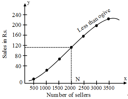
The value \(\frac{N}{2}\) = 115 is marked on y-axis and a line parallel to x-axis is drawn. This line meets the curve at a point P. From P draw a perpendicular PN to meet x-axis at median. Median = 2000.
Hence, the median of given frequency distribution is 2000.
Example 3: Draw the two ogives for the following frequency distribution of the weekly wages of (less than and more than) number of workers.
| Weekly wages | Number of workers |
| 0 – 20 | 41 |
| 20 – 40 | 51 |
| 40 – 60 | 64 |
| 60 – 80 | 38 |
| 80 – 100 | 7 |
Hence find the value of median.
Solution:
| Weekly wages | Number of workers | C.F (less than) | C.F (More than) |
| 0 – 20 | 41 | 41 | 201 |
| 20 – 40 | 51 | 92 | 160 |
| 40 – 60 | 64 | 156 | 109 |
| 60 – 80 | 38 | 194 | 45 |
| 80 – 100 | 7 | 201 | 7 |
Less than curve :
Upper limits of class intervals are marked on the x-axis and less than type cumulative frequencies are taken on y-axis. For drawing less than type curve, points (20, 41), (40, 92), (60, 156), (80, 194), (100, 201) are plotted on the graph paper and these are joined by free hand to obtain the less than ogive.
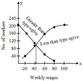
Greater than ogive
Lower limits of class interval are marked on x-axis and greater than type cumulative frequencies are taken on y-axis. For drawing greater than type curve, points (0, 201), (20, 160), (40, 109), (60, 45) and (80, 7) are plotted on the graph paper and these are joined by free hand to obtain the greater than type ogive. From the point of intersection of these curves a perpendicular line on x-axis is drawn. The point at which this line meets x-axis determines the median. Here the median is 42.652.
Example 4: Following table gives the cumulative frequency of the age of a group of 199 teachers.
Draw the less than ogive and greater than ogive and find the median.
| Age in years | Cum. Frequency |
| 20 – 25 | 21 |
| 25 – 30 | 40 |
| 30 – 35 | 90 |
| 35 – 40 | 130 |
| 40 – 45 | 146 |
| 45 – 50 | 166 |
| 50 – 55 | 176 |
| 55 – 60 | 186 |
| 60 – 65 | 195 |
| 65 – 70 | 199 |
Solution:
| Age in years | Less than cumulative frequency | Frequency | Greater than type |
| 20 – 25 | 21 | 21 | 199 |
| 25 – 30 | 40 | 19 | 178 |
| 30 – 35 | 90 | 50 | 159 |
| 35 – 40 | 130 | 40 | 109 |
| 40 – 45 | 146 | 16 | 69 |
| 45 – 50 | 166 | 20 | 53 |
| 50 – 55 | 176 | 10 | 33 |
| 55 – 60 | 186 | 10 | 23 |
| 60 – 65 | 195 | 9 | 13 |
| 65 – 70 | 199 | 4 | 4 |
Find out the frequencies by subtracting previous frequency from the next frequency to get simple frequency. Now we can prepare the greater than type frequency. Ages are taken on x-axis and number of teachers on y-axis.
Less than ogive :
Plot the points (25, 21), (30, 40), (35, 90), (40, 130), (45, 146), (50, 166), (55, 176), (60, 186), (65, 195), (70, 199) on graph paper. Join these points free hand to get less than ogive.
Greater than ogive :
Plot the points (20, 199), (25, 178), (30, 159), (35, 109), (40, 69), (45, 53), (50, 33), (55, 23), (60, 13), (65, 4) on graph paper. Join these points freehand to get greater than ogive. Median is the point of intersection of these two curves.
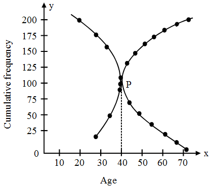
Here median is 37.375.
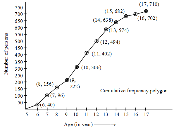
Example 5: Following is the age distribution of a group of students. Draw the cumulative frequency polygon, cumulative frequency curve (less than type) and hence obtain the median value.
| Age | Frequency |
| 5 – 6 | 40 |
| 6 – 7 | 56 |
| 7 – 8 | 60 |
| 8 – 9 | 66 |
| 9 – 10 | 84 |
| 10 – 11 | 96 |
| 11 – 12 | 92 |
| 12 – 13 | 80 |
| 13 – 14 | 64 |
| 14 – 15 | 44 |
| 15 – 16 | 20 |
| 16 – 17 | 8 |
Solution: We first prepare the cumulative frequency table by less then method as given below :
| Age | Frequency | Age less than | Cumulative frequency |
| 5 – 6 | 40 | 6 | 40 |
| 6 – 7 | 56 | 7 | 96 |
| 7 – 8 | 60 | 8 | 156 |
| 8 – 9 | 66 | 9 | 222 |
| 9 – 10 | 84 | 10 | 306 |
| 10 – 11 | 96 | 11 | 402 |
| 11 – 12 | 92 | 12 | 494 |
| 12 – 13 | 80 | 13 | 574 |
| 13 – 14 | 64 | 14 | 638 |
| 14 – 15 | 44 | 15 | 682 |
| 15 – 16 | 20 | 16 | 702 |
| 16 – 17 | 8 | 17 | 710 |
Other than the given class intervals, we assume a class 4-5 before the first class interval 5-6 with zero frequency.
Now, we mark the upper class limits (including the imagined class) along X-axis on a suitable scale and the cumulative frequencies along Y-axis on a suitable scale.
Thus, we plot the points (5, 0), (6, 40), (7, 96), (8, 156), (9, 222), (10, 306), (11, 402), (12, 494), (13, 574), (14, 638), (15, 682), (16, 702) and (17, 710).
These points are marked and joined by line segments to obtain the cumulative frequency polygon shown in Fig.
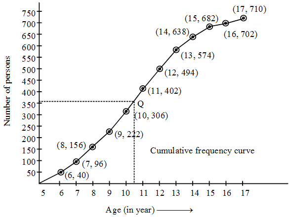
In order to obtain the cumulative frequency curve, we draw a smooth curve passing through the points discussed above. The graph (fig) shows the total number of students as 710. The median is the age corresponding to \(\frac{N}{2}\,\, = \,\,\frac{{710}}{2}\) = 355 students. In order to find the median, we first located the point corresponding to 355th student on Y-axis. Let the point be P. From this point draw a line parallel to the X-axis cutting the curve at Q. From this point Q draw a line parallel to Y-axis and meeting X-axis at the point M. The x-coordinate of M is 10.5 (See Fig.). Hence, median is 10.5.
Example 6: The following observations relate to the height of a group of persons. Draw the two type of cumulative frequency polygons and cumulative frequency curves and determine the median.
| Height in cms | 140–143 | 143–146 | 146–149 | 149–152 | 152–155 | 155–158 | 158–161 |
| Frequency | 3 | 9 | 26 | 31 | 45 | 64 | 78 |
| Height in cms | 161–164 | 164–167 | 167–170 | 170–173 | 173–176 | 176–179 | 179–182 |
| Frequency | 85 | 96 | 72 | 60 | 43 | 20 | 6 |
Solution: Less than method : We first prepare the cumulative frequency table by less than method as given below :
| Height in cms | Frequency | Height less than | Frequency |
| 140–143 | 3 | 143 | 3 |
| 143–146 | 9 | 146 | 12 |
| 146–149 | 26 | 149 | 38 |
| 149–152 | 31 | 152 | 69 |
| 152–155 | 45 | 155 | 114 |
| 155–158 | 64 | 158 | 178 |
| 158–161 | 78 | 161 | 256 |
| 161–164 | 85 | 164 | 341 |
| 164–167 | 96 | 167 | 437 |
| 167–170 | 72 | 170 | 509 |
| 170–173 | 60 | 173 | 569 |
| 173–176 | 43 | 176 | 612 |
| 176–179 | 20 | 179 | 632 |
| 179–182 | 6 | 182 | 638 |
Other than the given class intervals, we assume a class interval 137-140 prior to the first class interval 140-143 with zero frequency.
Now, we mark the upper class limits on X-axis and cumulative frequency along Y-axis on a suitable scale.
We plot the points (140, 0), (143, 3), (146, 12), (149, 38), (152, 69), (155, 114), (158, 178), (161, 256),
(164, 341), (167, 437), (170, 509), (173, 569), (176, 612),.(179, 632) and 182, 638).
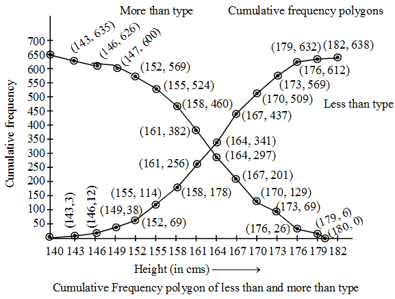
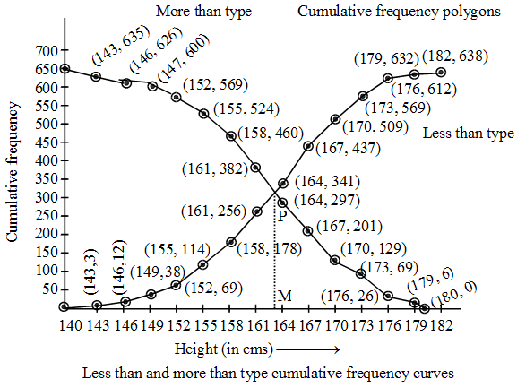
These points are joined by line segments to obtain the cumulative frequency polygon as shown in fig. and by a free hand smooth curve to obtain an ogive by less than method as shown in fig.
More than method : We prepare the cumulative frequency table by more than method as given below :
Other than the given class intervals, we assume the class interval 182-185 with zero frequency.
Now, we mark the lower class limits on X-axis and the cumulative frequencies along Y-axis on suitable scales to plot the points (140, 638), (143, 635), (146, 626), (149, 600), (152, 569), (155, 524), (158, 460), (161, 382), (164, 297), (167, 201), (170, 129), (173, 69), (176, 26) and (179, 6). By joining these points by line segments, we obtain the more than type frequency polygon as shown in fig. By joining these points by a free hand curve, we obtain more than type cumulative frequency curve as points by a free hand curve, we obtain more than type cumulative frequency curves as shown in fig.
We find that the two types of cumulative frequency curves intersect at point P. From point P perpendicular PM is drawn on X-axis. The value of height corresponding to M is 163.2 cm. Hence, median is 163.2 cm.