Normal Distribution
A normal distribution is a very important statistical data distribution pattern occurring in many natural phenomena, such as height, blood pressure, lengths of objects produced by machines, etc. Certain data, when graphed as a histogram (data on the horizontal axis, amount of data on the vertical axis), creates a bell-shaped curve known as a normal curve, or normal distribution.
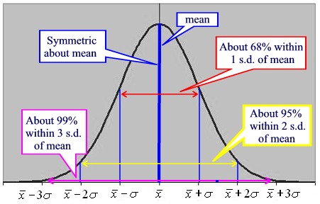
Normal distributions are symmetrical with a single central peak at the mean (average) of the data. The shape of the curve is described as bell-shaped with the graph falling off evenly on either side of the mean. Fifty percent of the distribution lies to the left of the mean and fifty percent lies to the right of the mean.
The spread of a normal distribution is controlled by the standard deviation. The smaller the standard deviation the more concentrated the data.
The mean and the median are the same in a normal distribution.
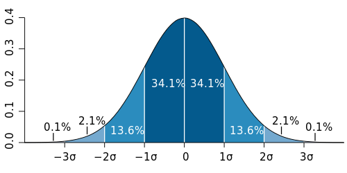
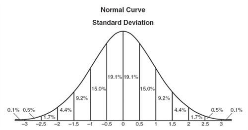 Reading from the chart, we see that approximately 19.1% of normally distributed data is located between the mean (the peak) and 0.5 standard deviations to the right (or left) of the mean.
(The percentages are represented by the area under the curve.)
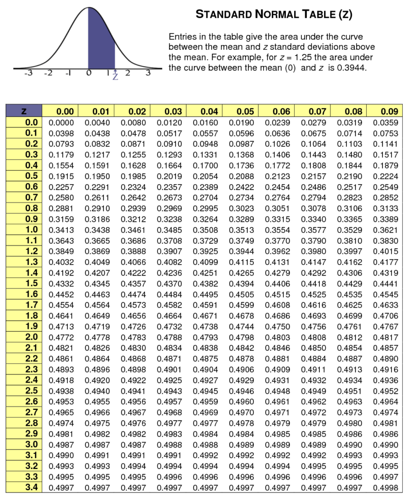
Understand that this chart shows only percentages that correspond to subdivisions up to one-half of one standard deviation. Percentages for other subdivisions require a statistical mathematical table or a graphing calculator. (See example 4)
If you add percentages, you will see that approximately:
- 68% of the distribution lies within one standard deviation of the mean.
- 95% of the distribution lies within two standard deviations of the mean.
- 99.7% of the distribution lies within three standard deviations of the mean.
These percentages are known as the “empirical rule“.
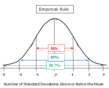 Note: The addition of percentages in the chart at the top of the page are slightly different than the empirical rule values due to rounding that has occurred in the chart.
 It is also true that: 50% of the distribution lies within 0.67448 standard deviations of the mean.
If you are asked for the interval about the mean containing 50% of the data, you are actually being asked for the interquartile range, IQR. The IQR (the width of an interval which contains the middle 50% of the data set) is normally computed by subtracting the first quartile from the third quartile. In a normal distribution (with mean 0 and standard deviation 1), the first and third quartiles are located at -0.67448 and +0.67448 respectively. Thus the IQR for a normal distribution is:
QR = Q3 – Q1 = 2(0.67448) x σ = 1.34986 σ
Interquartile range = 1.34896 x standard deviation
(this will be the population IQR)
Percentiles and the Normal Curve
The mean (at the center peak of the curve) is the 50% percentile.
The term “percentile rank” refers to the area (probability) to the left of the value.
Adding the given percentages from the chart will let you find certain percentiles along the curve.
Examples: Look for the words “normally distributed” in a question before referring to the Normal Distribution Standard Deviation chart seen on this page. When using the chart, your information should fall on the increments of one-half of one standard deviation as shown in the chart.
1. Find the percentage of the normally distributed data that lies within 2 standard deviations of the mean.
Solution:
Read the percentages from the chart at the top of this page from -2 to +2 standard deviations.
4.4% + 9.2% + 15.0% + 19.1% + 19.1% + 15.0% + 9.2% + 4.4% = 95.4%
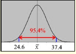
2. At the New Age Information Corporation, the ages of all new employees hired during the last 5 years are normally distributed. Within this curve, 95.4% of the ages, centered about the mean, are between 24.6 and 37.4 years. Find the mean age and the standard deviation of the data.
Solution:
As was seen in Example 1, 95.4% implies a span of 2 standard deviations from the mean. The mean age is symmetrically located between -2 standard deviations (24.6) and +2 standard deviations (37.4).
The mean age is 24.6+37.4/2 years of age.
From 31 to 37.4 (a distance of 6.4 years) is 2 standard deviations. Therefore, 1 standard deviation is (6.4)/2 = 3.2 years.
3. The amount of time that Carlos plays video games in any given week is normally distributed. If Carlos plays video games an average of 15 hours per week, with a standard deviation of 3 hours, what is the probability of Carlos playing video games between 15 and 18 hours a week?
Solution: The average (mean) is 15 hours. If the standard deviation is 3, the interval between 15 and 18 hours is one standard deviation above the mean, which gives a probability of 34.1% or 0.341, as seen in the chart at the top of this page.